Visual search over an image library

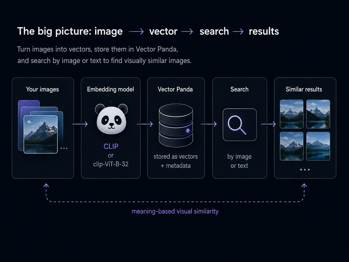
You have a folder of images on your laptop. Maybe it's product photos, design references, screenshots, scanned artwork, anything visual. You'd like to type "woman in a black dress" and get the matching pictures back, or hand the system a photo and find the visually similar ones.

This project walks through it end to end with a real corpus you can either build yourself or download. We use ~45 famous Metropolitan Museum of Art works (Van Gogh's Wheat Field, Sargent's Madame X, Hokusai's Great Wave, Vermeer, Rembrandt, the Temple of Dendur) because they're real, public-domain, instantly recognizable, and small enough to run in a couple of minutes. Once you've finished, the only line to change for your own data is the folder path.

What you need

• Python 3.9 or newer
• About 5 minutes for setup, 25 minutes to run end to end (CLIP downloads ~600 MB on first call)
• An internet connection (to fetch the example corpus, to download the embedding model on first run, and to talk to Vector Panda)

pip install veep[pandas,parquet] sentence-transformers pillow

pip install langchain-vectorpanda langchain-huggingface veep[pandas,parquet] sentence-transformers pillow

veep[pandas,parquet] is the SDK plus pandas and pyarrow. sentence-transformers is the local embedding library; pillow is the image-loading library it uses to read your JPEGs and PNGs. Nothing leaves your machine until you upload to Vector Panda.

Get the corpus

We need a folder of images to make searchable. Two ways to get one; pick whichever you prefer.

A. Build it yourself (recommended)

This way you watch the data come in, see what each row looks like, and the only thing you change for your own data is the source of the images. The Met's Open Access API has no key and no rate limit beyond basic politeness; we'll hit it directly.

import json, pathlib, time, urllib.request

# A handful of recognizable Met holdings. Each entry is a Met objectID
# (browse the catalog at https://www.metmuseum.org/art/collection; the URL
# slug ends in the ID). Extend this list with anything you'd like to search.
OBJECT_IDS = [
    436535,  # Van Gogh — Wheat Field with Cypresses
    12127,   # Sargent — Madame X
    11417,   # Leutze — Washington Crossing the Delaware
    39799,   # Hokusai — Great Wave off Kanagawa
    438817,  # Degas — The Dance Class
    547802,  # Temple of Dendur
    436105,  # David — Death of Socrates
    435868,  # Cézanne — The Card Players
]

out = pathlib.Path("met-famous")
img_dir = out / "img"
img_dir.mkdir(parents=True, exist_ok=True)

ua = {"User-Agent": "VeepBYODExample/1.0 (you@example.com)"}
rows = []

for oid in OBJECT_IDS:
    req = urllib.request.Request(
        f"https://collectionapi.metmuseum.org/public/collection/v1/objects/{oid}",
        headers=ua,
    )
    with urllib.request.urlopen(req, timeout=20) as resp:
        obj = json.load(resp)
    img_url = obj.get("primaryImageSmall")
    if not img_url:
        continue  # some objects have no public image; skip them
    img_bytes = urllib.request.urlopen(
        urllib.request.Request(img_url, headers=ua), timeout=20,
    ).read()
    img_path = img_dir / f"{oid}.jpg"
    img_path.write_bytes(img_bytes)
    rows.append({
        "object_id": oid,
        "title": obj.get("title", ""),
        "artist": obj.get("artistDisplayName", ""),
        "image_file": f"img/{oid}.jpg",
    })
    time.sleep(0.5)  # be polite to the Met API

(out / "metadata.json").write_text(json.dumps(rows, indent=2))
print(f"wrote {len(rows)} images + metadata.json to {out}/")

You'll see something like:

wrote 8 images + metadata.json to met-famous/

Eight is enough to run the rest of the project end to end and watch the queries return on-target. If you want the larger corpus we used to write this guide (~45 works, the same shape), use option B below; everything that follows runs identically against either.

B. Or skip the wait

Pre-bundled, same shape. Useful if you don't want to wait or you're behind a firewall that blocks the Met API.

import tarfile, urllib.request

urllib.request.urlretrieve(
    "https://next.vectorpanda.com/data/example-met-famous.tar.gz",
    "met-famous.tar.gz",
)
with tarfile.open("met-famous.tar.gz") as tf:
    tf.extractall(".")
print("extracted to met-famous/")

Either way you should now have a met-famous/ folder with img/ (one JPEG per work) and metadata.json. Open metadata.json in your editor; it's just a list of {object_id, title, artist, image_file} rows. That's all the structure we need.

Vector Panda doesn't open images, doesn't read metadata, doesn't store the file. The image is just bytes we'll feed to the embedder; what lands in Vector Panda is the resulting vector plus whatever metadata you choose to send.

Embed your corpus

Now turn each image into a vector. We'll use clip-ViT-B-32, the OpenAI CLIP model packaged for sentence-transformers. CLIP is special: it embeds both images and text into the same 512-dimensional space, which is what lets you query images with typed sentences a few sections from now. Vector Panda is model-agnostic; bring whatever you'd like.

import json, pathlib
from PIL import Image
from sentence_transformers import SentenceTransformer

model = SentenceTransformer("clip-ViT-B-32")  # ~600 MB download on first call

meta = json.loads(pathlib.Path("met-famous/metadata.json").read_text())
images = [Image.open(f"met-famous/{row['image_file']}") for row in meta]

embeddings = model.encode(images, show_progress_bar=True, normalize_embeddings=True)
print(f"embedded {len(embeddings)} images; vector dim = {embeddings.shape[1]}")

After a progress bar, you'll see:

embedded 45 images; vector dim = 512

(Or 8 if you took the build-it-yourself path.) Every image is now a list of 512 floats. clip-ViT-B-32 is a 512-dimensional model; if you swap models, this number changes. Vector Panda doesn't care which dimensionality you pick, as long as your query vectors match what you uploaded.

We passed normalize_embeddings=True because cosine similarity (Vector Panda's default metric) wants unit-length vectors. CLIP's raw output is unnormalized; one flag fixes that. See Cosine similarity vs Euclidean distance for why this matters.

You now have a parallel list of (metadata row, vector) pairs. Time to put them in Vector Panda.

Upload and query

This is where you pick your input shape. Each tab is a complete walkthrough; pick the one that matches how you'd naturally structure your own data, copy-paste, and run. The query at the end is the same regardless.

import pandas as pd
from veep import VP

df = pd.DataFrame({
    "id": [str(row["object_id"]) for row in meta],
    "vector": [e.tolist() for e in embeddings],
    "title": [row["title"] for row in meta],
    "artist": [row["artist"] for row in meta],
})
df.to_parquet("met-famous.parquet", index=False)

vp = VP.from_creds()
vp.collections.create("met-from-parquet", tier="hot")
vp.vectors.upsert("met-from-parquet", "met-famous.parquet")

q = model.encode("a painting of dancers", normalize_embeddings=True).tolist()
results = vp.vectors.query("met-from-parquet", vector=q, top_k=3)
for r in results:
    print(f"{r.score:.3f}  {r.metadata.get('title', '?')}  —  {r.metadata.get('artist', '?')}")

import pandas as pd
from veep import VP

df = pd.DataFrame({
    "id": [str(row["object_id"]) for row in meta],
    "vector": [e.tolist() for e in embeddings],
    "title": [row["title"] for row in meta],
    "artist": [row["artist"] for row in meta],
})

vp = VP.from_creds()
vp.collections.create("met-from-dataframe", tier="hot")
vp.vectors.upsert("met-from-dataframe", dataframe=df)

q = model.encode("a painting of dancers", normalize_embeddings=True).tolist()
results = vp.vectors.query("met-from-dataframe", vector=q, top_k=3)
for r in results:
    print(f"{r.score:.3f}  {r.metadata.get('title', '?')}  —  {r.metadata.get('artist', '?')}")

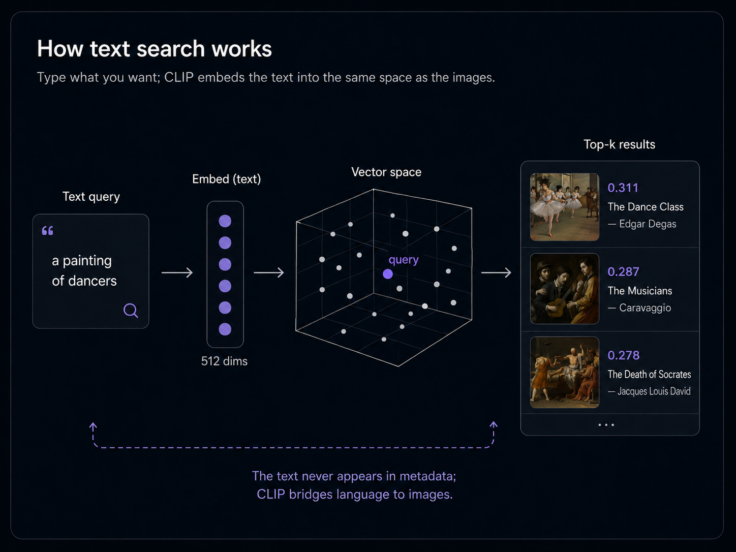
If your query was "a painting of dancers", the top result should be Degas. Sample output from the parquet path on the full ~45-work corpus:

0.311  The Dance Class  —  Edgar Degas
0.287  The Musicians  —  Caravaggio (Michelangelo Merisi)
0.278  The Death of Socrates  —  Jacques Louis David

Embeddings aren't deterministic across machines, so the exact ranking varies, but the matches will be sensible. The thing to notice: nothing in the metadata uses the word "dancer." The match is purely visual; CLIP saw a painting of figures in motion and ranked Degas first, with two other multi-figure compositions behind it.

Using LangChain instead

The pre-computed image embeddings go through veep directly (LangChain's text-first add_texts would re-embed). Wrap the populated collection in VectorPandaStore and the text-query path becomes a one-liner — the same CLIP model handles both image embedding (above) and text embedding (in the store).

from langchain_huggingface import HuggingFaceEmbeddings
from langchain_vectorpanda import VectorPandaStore

embedder = HuggingFaceEmbeddings(model_name="clip-ViT-B-32")  # same CLIP model
store = VectorPandaStore(
    collection_name="met-from-parquet",  # or met-from-dataframe
    embedding=embedder,
    client=vp,
)

# Text query: the store embeds via CLIP's text encoder.
for doc, score in store.similarity_search_with_score("a painting of dancers", k=3):
    print(f"{score:.3f}  {doc.metadata.get('title', '?')}  —  {doc.metadata.get('artist', '?')}")

Image queries (next section) stay on the manual model.encode(image) path and call store.similarity_search_by_vector_with_score(...) — the LangChain VectorStore interface is text-oriented, but the by-vector path lets you pass any embedding you computed yourself.

A note on the absolute numbers: cross-modal CLIP scores cluster in the 0.2 to 0.4 range. That's lower than the 0.6 to 0.8 you'll see when both sides are text or both sides are images, because CLIP's text encoder and image encoder are aligned rather than identical. Don't read 0.31 as a weak match; it's a strong signal in this regime. What matters is the ranking.

Try a few more text queries and watch how the meaning carries through. We'll set up one more collection from the same vectors so this section is self-contained, runnable whether or not you stuck with the tab above:

import pandas as pd

df = pd.DataFrame({
    "id": [str(row["object_id"]) for row in meta],
    "vector": [e.tolist() for e in embeddings],
    "title": [row["title"] for row in meta],
    "artist": [row["artist"] for row in meta],
})
vp.collections.create("met-bonus", tier="hot")
vp.vectors.upsert("met-bonus", dataframe=df)

for query in [
    "a cresting ocean wave",
    "an ancient egyptian temple",
    "a portrait of a woman in a black dress",
    "soldiers in a boat at war",
    "a horse in a field",
]:
    print(f"\n>>> {query}")
    q = model.encode(query, normalize_embeddings=True).tolist()
    for r in vp.vectors.query("met-bonus", vector=q, top_k=3):
        print(f"  {r.score:.3f}  {r.metadata.get('title', '?')[:55]}")

import pandas as pd

df = pd.DataFrame({
    "id": [str(row["object_id"]) for row in meta],
    "vector": [e.tolist() for e in embeddings],
    "title": [row["title"] for row in meta],
    "artist": [row["artist"] for row in meta],
})
vp.collections.create("met-bonus-lc", tier="hot")
vp.vectors.upsert("met-bonus-lc", dataframe=df)

bonus = VectorPandaStore(
    collection_name="met-bonus-lc",
    embedding=embedder,  # the HuggingFaceEmbeddings("clip-ViT-B-32") from above
    client=vp,
)

for query in [
    "a cresting ocean wave",
    "an ancient egyptian temple",
    "a portrait of a woman in a black dress",
    "soldiers in a boat at war",
    "a horse in a field",
]:
    print(f"\n>>> {query}")
    for doc, score in bonus.similarity_search_with_score(query, k=3):
        print(f"  {score:.3f}  {doc.metadata.get('title', '?')[:55]}")

You'll see something like:

>>> a cresting ocean wave
  0.270  Under the Wave off Kanagawa (Kanagawa oki nami ura), or
  0.214  Whalers
  0.209  Guqin (古琴 )

>>> an ancient egyptian temple
  0.311  The Temple of Dendur
  0.219  The Death of Socrates
  0.216  Bronze chariot inlaid with ivory

>>> a portrait of a woman in a black dress
  0.343  Madame X (Virginie Amélie Avegno Gautreau)
  0.288  Young Lady in 1866
  0.270  Juan de Pareja (ca. 1608–1670)

>>> soldiers in a boat at war
  0.318  Whalers
  0.315  The Gulf Stream
  0.280  Fur Traders Descending the Missouri

>>> a horse in a field
  0.276  Whalers
  0.275  The Horse Fair
  0.258  Wheat Field with Cypresses

These are scores from a run on the day this guide was written. Yours will be slightly different, but the same general matches should land in the top three. The text never appears in the corpus metadata; CLIP is doing the work of bridging "ocean wave" to Hokusai and "woman in a black dress" to Sargent.

Two of these queries are worth a closer look. "Soldiers in a boat at war" returned Whalers (Turner) ahead of Washington Crossing the Delaware (the obvious target, which didn't crack the top three at all). CLIP latched onto "men in a boat on rough water" more strongly than "battle at war." And "a horse in a field" tied Whalers with The Horse Fair at 0.276 vs 0.275; the Horse Fair has the right subject, but Whalers happened to have the wider, calmer composition CLIP associates with "field." This is what real CLIP behavior looks like. The model is unbiased and surprisingly good, but it isn't a reasoner.

Search by image, not text

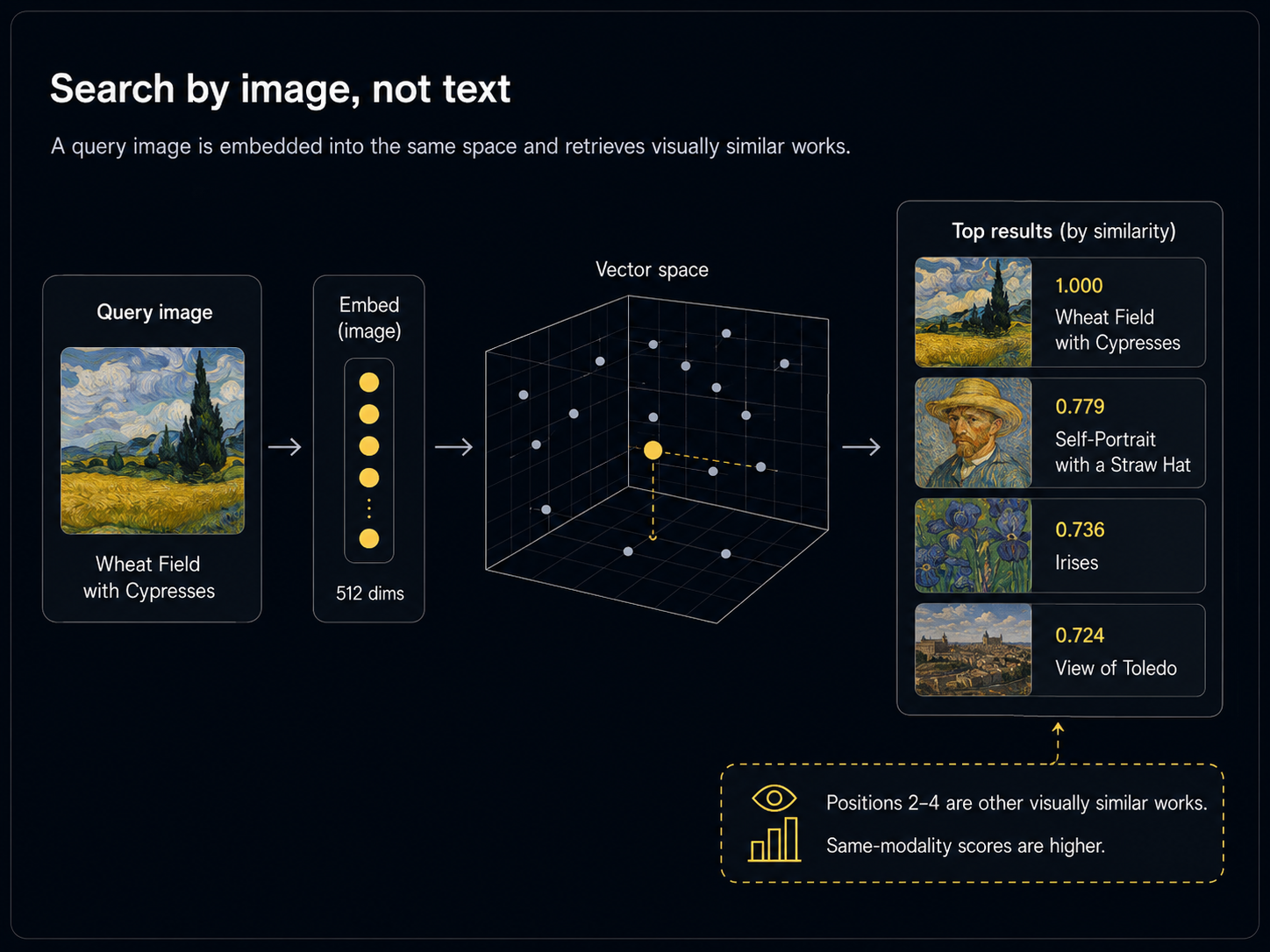
CLIP's same-space trick goes both directions. You can hand it an image and ask for the most visually similar ones in the collection. The query vector is just a different call to the same model.encode().

Pick any image in the corpus as the query (or one of your own); we'll use the Wheat Field as an example. The top result will be the image itself (cosine similarity 1.0), so look at positions 2 onward.

from PIL import Image

query_img = Image.open("met-famous/img/436535.jpg")  # Van Gogh, Wheat Field
q = model.encode(query_img, normalize_embeddings=True).tolist()

results = vp.vectors.query("met-bonus", vector=q, top_k=5)
for r in results:
    print(f"  {r.score:.3f}  {r.metadata.get('title', '?')[:55]}  —  {r.metadata.get('artist', '?')}")

from PIL import Image

query_img = Image.open("met-famous/img/436535.jpg")  # Van Gogh, Wheat Field
q = model.encode(query_img, normalize_embeddings=True).tolist()

# LangChain's VectorStore interface is text-oriented; image queries take
# the precomputed-vector path.
results = bonus.similarity_search_by_vector_with_score(q, k=5)
for doc, score in results:
    print(f"  {score:.3f}  {doc.metadata.get('title', '?')[:55]}  —  {doc.metadata.get('artist', '?')}")

You'll see something like:

  1.000  Wheat Field with Cypresses                              —  Vincent van Gogh
  0.779  Self-Portrait with a Straw Hat (obverse: The Potato P  —  Vincent van Gogh
  0.736  Irises                                                  —  Vincent van Gogh
  0.724  View of Toledo                                          —  El Greco
  0.699  The Englishman (William Tom Warrener, 1861–1934) at t  —  Henri de Toulouse-Lautrec

Position 1 is the query image itself. Positions 2–4 are the other three Van Goghs in the corpus, ranked by visual similarity (the Self-Portrait shares the same yellow-and-blue palette and visible brushwork; Irises shares the impasto). Position 5 jumps to El Greco's View of Toledo, which has the same brooding sky and tilted horizon, then Toulouse-Lautrec, who shares the late-19th-century painterly handling. CLIP isn't reasoning about "Van Gogh as an artist"; it's picking up on color, composition, and paint texture, and that ends up clustering Van Gogh tightly anyway.

Notice how much higher the scores are here (0.7 to 0.8) than the cross-modal text queries above (0.2 to 0.3). Same-modality search is just easier; CLIP doesn't need to bridge between two encoders. If your application is image-only search, expect the higher range.

Drop in any image you have on hand (a photo, a screenshot, a magazine page) as the query. Just point Image.open at the path. Here's Madame X used as the query for a second look, which pulls other portraits of women toward the top:

query_img = Image.open("met-famous/img/12127.jpg")  # Sargent, Madame X
q = model.encode(query_img, normalize_embeddings=True).tolist()
for r in vp.vectors.query("met-bonus", vector=q, top_k=5):
    print(f"  {r.score:.3f}  {r.metadata.get('title', '?')[:55]}")

query_img = Image.open("met-famous/img/12127.jpg")  # Sargent, Madame X
q = model.encode(query_img, normalize_embeddings=True).tolist()
for doc, score in bonus.similarity_search_by_vector_with_score(q, k=5):
    print(f"  {score:.3f}  {doc.metadata.get('title', '?')[:55]}")

  1.000  Madame X (Virginie Amélie Avegno Gautreau)
  0.793  Young Lady in 1866
  0.774  Madame Georges Charpentier (Marguerite-Louise Lemonnier
  0.721  Young Woman with a Water Pitcher
  0.714  The Dance Class

Position 1 is Madame X herself. Positions 2 to 4 are three other female portraits (Manet's Young Lady, Renoir's Madame Charpentier, Vermeer's Young Woman with a Water Pitcher). Position 5 is the Dance Class, which is also a multi-figure painting with women in it. CLIP picked "portrait of a woman" without anyone telling it that's what we wanted.

The match quality on out-of-distribution images (your own photos) depends on how close they are visually to anything in the corpus. CLIP was trained on hundreds of millions of (image, caption) pairs from the web, so it has surprisingly broad coverage; it just won't know that the photo on your phone is "you on vacation in Greece" the way it knows Van Gogh.

Now what

You just built a visual search engine over your own images, queryable by typed sentence or by another image. The pattern works for anything that's "files of pictures": product photography, design references, scanned artwork, screenshots, satellite tiles, frames extracted from video.

To make it yours:

1. Replace the met-famous/ folder with a folder of your own images.
2. The metadata is whatever fits your data: SKU + price for products, project + tag for designs, capture date for photos. Vector Panda stores whatever you put in the DataFrame.
3. CLIP works well on natural photographs and most artwork. For more specialized domains (medical imaging, satellite, faces), a domain-tuned model will usually beat it.
4. If you want both text-search and image-search over the same corpus (e.g., product photos with descriptions), embed each image with CLIP and store one row per item. Both query types hit the same collection.

Read the SDK reference for everything vp.vectors.upsert() and vp.vectors.query() can do. The embeddings 101 concept page explains the geometry behind why typing "ocean wave" finds Hokusai.