
You run a streaming site. A user has watched five films, and they liked all of them. You'd like to surface another ten they probably also want to watch, but not just "more of the last thing they clicked." Something that captures the blend of what they're into.
This project walks through the pattern end to end with the bundled 5,000-film movie corpus that ships with veep[samples] (the same dataset the quickstart on /docs uses). Once you've finished, the only line to change to plug in your own catalogue is the source DataFrame.
The trick is one of the things vector databases are uniquely good at: vector arithmetic. Take the embedding of each film a user has watched, average the vectors, renormalize, and use that as the query. The result is a single point in the same 384-dimensional space that represents the user's "taste." Cosine-nearest neighbours to that point are the recommendations.
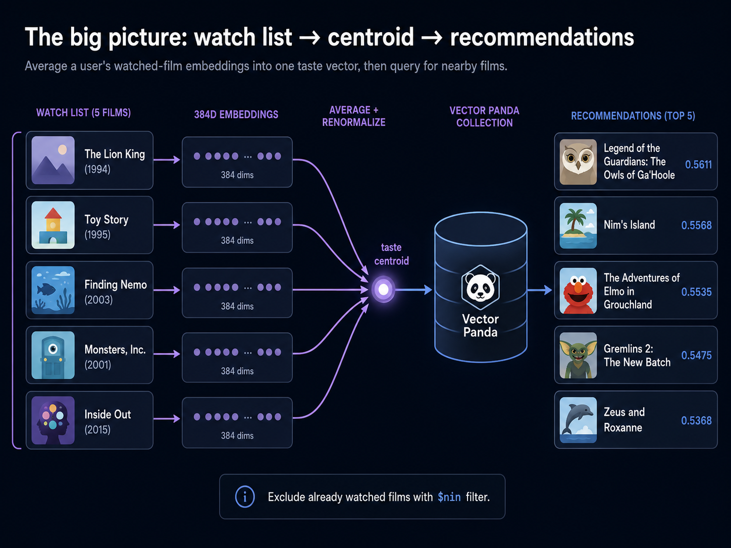
What you need
- Python 3.9 or newer
- About 5 minutes for setup, 15 minutes to run end to end
- An internet connection (to talk to Vector Panda; the corpus is already bundled)
pip install veep[samples,pandas,parquet] numpy
pip install langchain-vectorpanda langchain-huggingface veep[samples,pandas,parquet] numpy
langchain-huggingface (which pulls sentence-transformers and torch) is only needed if you'll do text-search later; this walkthrough is by-vector throughout, so you can skip it if your project doesn't need a text path.
The [samples] extra adds the 5,000-film movie DataFrame. numpy is what we'll use to average vectors. Nothing leaves your machine until you upload to Vector Panda.
Upload the corpus
The bundled DataFrame has six columns: id, title, year, genre, plot, vector. The id column becomes the row key on upsert; the rest become filterable metadata.
from veep import VP, samples

df = samples.dataframe()

vp = VP.from_creds()
vp.collections.create("movie-recs", tier="hot")
vp.vectors.upsert("movie-recs", dataframe=df)

print(f"uploaded {len(df)} films; vector dim = {len(df.iloc[0].vector)}")
The bundled DataFrame ships with pre-computed embeddings, so the upload itself goes through veep directly — LangChain's VectorStore.add_texts is text-first and would re-embed every plot. Wrap the populated collection in VectorPandaStore once the upsert is done and the rest of this walkthrough is pure LangChain.
from veep import VP, samples
from langchain_huggingface import HuggingFaceEmbeddings
from langchain_vectorpanda import VectorPandaStore

df = samples.dataframe()

vp = VP.from_creds()
vp.collections.create("movie-recs", tier="hot")
vp.vectors.upsert("movie-recs", dataframe=df)

# Match the embedding model the bundled DataFrame was built with.
# Used only for text-query paths; similarity_search_by_vector skips it.
embeddings = HuggingFaceEmbeddings(
    model_name="sentence-transformers/all-MiniLM-L6-v2"
)
store = VectorPandaStore(
    collection_name="movie-recs",
    embedding=embeddings,
    client=vp,
)

print(f"uploaded {len(df)} films; vector dim = {len(df.iloc[0].vector)}")
You'll see:
uploaded 5000 films; vector dim = 384
Build a watch list and a taste centroid
Pick five films a fake user has watched recently. We'll use a coherent theme so the recommendations are recognizable: animated family films from the late 90s through 2010s.
import numpy as np

WATCH_LIST = [
    "film-00002",  # The Lion King (1994)
    "film-00004",  # Toy Story (1995)
    "film-00026",  # Finding Nemo (2003)
    "film-00039",  # Monsters, Inc. (2001)
    "film-00042",  # Inside Out (2015)
]

# Look up each watched film's vector from the DataFrame.
# In a real app you'd vp.vectors.fetch() these from the collection, but
# we already have them in memory from the upsert.
watched_vectors = np.stack([
    np.array(df[df.id == fid].iloc[0].vector) for fid in WATCH_LIST
])
print(f"watched_vectors shape: {watched_vectors.shape}")

# Average the five vectors → the "taste centroid."
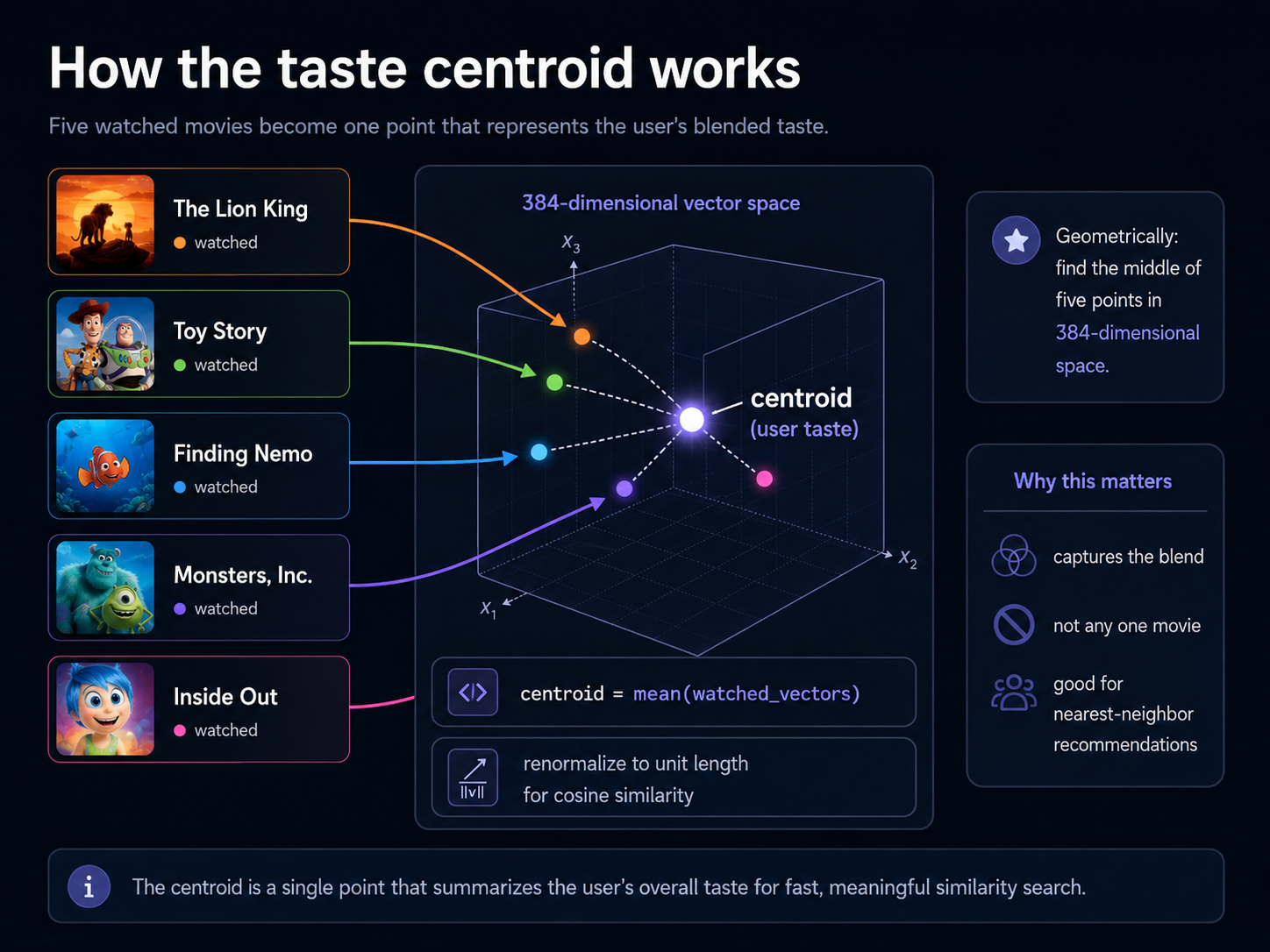
centroid = watched_vectors.mean(axis=0)

# Renormalize to unit length. Cosine similarity treats vectors as directions,
# so the centroid's magnitude doesn't matter, but the SDK and most embedding
# models work best with unit-length vectors.
centroid = centroid / np.linalg.norm(centroid)
print(f"centroid: {len(centroid)} dims, |v| = {np.linalg.norm(centroid):.3f}")
watched_vectors shape: (5, 384)
centroid: 384 dims, |v| = 1.000
Geometrically, you've taken five points in a 384-dimensional space and found their middle. That middle is the user's "taste": not literally any single watched film, but the direction in space that all five share.
Query with the centroid
Now query the collection using the centroid as the search vector. The $nin filter excludes the five films already on the watch list (otherwise they'd dominate the top results, since they're as close to the centroid as anything).
results = vp.vectors.query(
    "movie-recs",
    vector=centroid.tolist(),
    top_k=5,
    filter={"id": {"$nin": WATCH_LIST}},
)
for r in results:
    m = r.metadata
    print(f"  {r.score:.4f}  {m.get('title','?')[:40]:<40}  ({m.get('year','?')}, {m.get('genre','?')[:20]})")
results = store.similarity_search_by_vector_with_score(
    centroid.tolist(),
    k=5,
    filter={"id": {"$nin": WATCH_LIST}},
)
for doc, score in results:
    m = doc.metadata
    print(f"  {score:.4f}  {m.get('title','?')[:40]:<40}  ({m.get('year','?')}, {m.get('genre','?')[:20]})")
  0.5611  Legend of the Guardians: The Owls of Ga'  (2010, fantasy)
  0.5568  Nim's Island                              (2008, adventure)
  0.5535  The Adventures of Elmo in Grouchland      (1999, children's film)
  0.5475  Gremlins 2: The New Batch                 (1990, sci-fi comedy)
  0.5368  Zeus and Roxanne                          (1997, family)
These are real recommendations from a real run. The user's taste profile (Pixar/Disney-flavoured family films) pulled in more family-and-creature stories: an owl-fantasy adventure, a girl-and-her-island story, a Sesame Street film, a creature comedy, and a boy-and-his-dolphin film. The model never saw the word "Pixar" or "kids movie"; it's reading the plot embeddings and picking up on shared themes (small heroes, animals, adventure, warmth).
Combine the centroid with filters
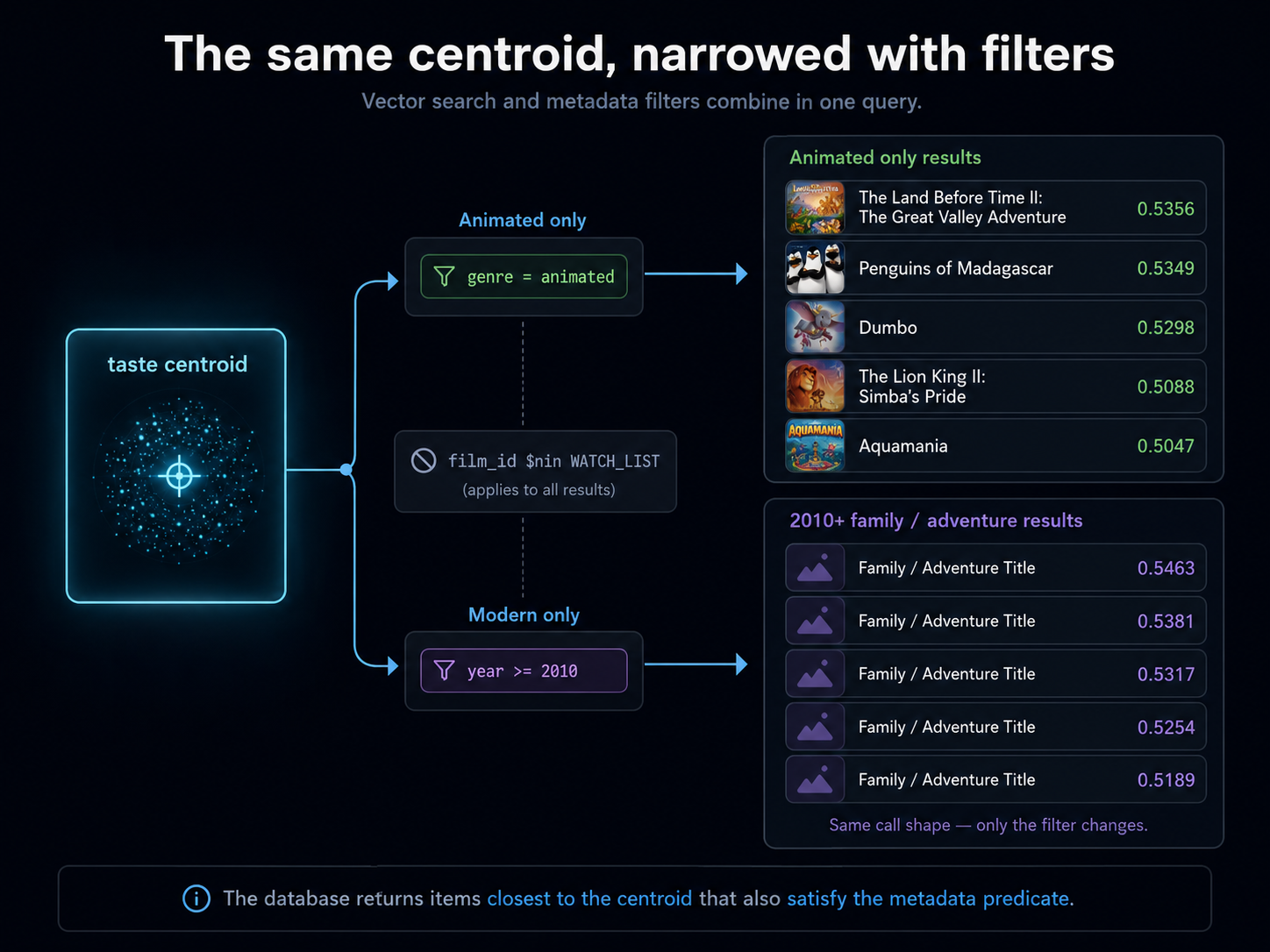
The same centroid plus a metadata filter scopes recommendations to a slice of the catalogue. Suppose the user wants only animated films:
results = vp.vectors.query(
    "movie-recs",
    vector=centroid.tolist(),
    top_k=5,
    filter={"id": {"$nin": WATCH_LIST}, "genre": "animated"},
)
for r in results:
    m = r.metadata
    print(f"  {r.score:.4f}  {m.get('title','?')[:40]:<40}  ({m.get('year','?')})")
results = store.similarity_search_by_vector_with_score(
    centroid.tolist(),
    k=5,
    filter={"id": {"$nin": WATCH_LIST}, "genre": "animated"},
)
for doc, score in results:
    m = doc.metadata
    print(f"  {score:.4f}  {m.get('title','?')[:40]:<40}  ({m.get('year','?')})")
  0.5356  The Land Before Time II: The Great Valle  (1994)
  0.5349  Penguins of Madagascar                    (2014)
  0.5298  Dumbo                                     (1941)
  0.5088  The Lion King II: Simba's Pride           (1998)
  0.5047  Aquamania                                 (1961)
Same centroid, narrower lens. The filter ANDs with the centroid query: the database returns the items closest to the centroid that also satisfy the metadata predicate. You can compose any of $eq, $ne, $in, $nin, $gt, $gte, $lt, $lte across as many fields as you like; everything has to be true for a row to qualify.
A second example: the same user wants something modern (2010 or later):
results = vp.vectors.query(
    "movie-recs",
    vector=centroid.tolist(),
    top_k=5,
    filter={"id": {"$nin": WATCH_LIST}, "year": {"$gte": 2010}},
)
for r in results:
    m = r.metadata
    print(f"  {r.score:.4f}  {m.get('title','?')[:40]:<40}  ({m.get('year','?')}, {m.get('genre','?')[:20]})")
results = store.similarity_search_by_vector_with_score(
    centroid.tolist(),
    k=5,
    filter={"id": {"$nin": WATCH_LIST}, "year": {"$gte": 2010}},
)
for doc, score in results:
    m = doc.metadata
    print(f"  {score:.4f}  {m.get('title','?')[:40]:<40}  ({m.get('year','?')}, {m.get('genre','?')[:20]})")
The shape of the call is identical; only the filter changes. This is the part of the design that customers usually want to see early: scoping a vector search to a structured slice is one operation, not two.
A second user, a different taste
To see the centroid trick really pay off, build a different user with a different watch list. This one's into epic fantasy:
WATCH_B = [
    "film-00023",  # The Lord of the Rings: The Fellowship of the Ring (2001)
    "film-00027",  # The Lord of the Rings: The Return of the King (2003)
    "film-00035",  # The Lord of the Rings: The Two Towers (2002)
    "film-00053",  # Harry Potter and the Deathly Hallows: Part 1 (2010)
    "film-00062",  # Harry Potter and the Deathly Hallows: Part 2 (2011)
]

vecs_b = np.stack([
    np.array(df[df.id == fid].iloc[0].vector) for fid in WATCH_B
])
centroid_b = vecs_b.mean(axis=0)
centroid_b = centroid_b / np.linalg.norm(centroid_b)
results = vp.vectors.query(
    "movie-recs",
    vector=centroid_b.tolist(),
    top_k=5,
    filter={"id": {"$nin": WATCH_B}},
)
for r in results:
    m = r.metadata
    print(f"  {r.score:.4f}  {m.get('title','?')[:40]:<40}  ({m.get('year','?')}, {m.get('genre','?')[:20]})")
results = store.similarity_search_by_vector_with_score(
    centroid_b.tolist(),
    k=5,
    filter={"id": {"$nin": WATCH_B}},
)
for doc, score in results:
    m = doc.metadata
    print(f"  {score:.4f}  {m.get('title','?')[:40]:<40}  ({m.get('year','?')}, {m.get('genre','?')[:20]})")
  0.5267  The Secret of the Sword                   (1985, animation)
  0.4897  Hercules in the Haunted World             (1961, adventure)
  0.4895  King Arthur: Legend of the Sword          (2017, action, adventure, e)
  0.4770  Smurfs: The Lost Village                  (2017, animation, comedy, f)
  0.4691  Hellboy II: The Golden Army               (2008, action, superhero)
A 1985 sword-fantasy animation, two different epic-quest films (Hercules, King Arthur), a family animation with a quest plot, and a supernatural-action film. The centroid's blending the LOTR axis (long quest, magic, swords, dark forces) with the Harry Potter axis (magic, school, dark forces, friends) and pulling out other "small band on an epic quest against magical evil" stories. None of them were in the watch list and none are obvious sequels; the database is doing real recommendation work.
Why the centroid beats single-item similarity
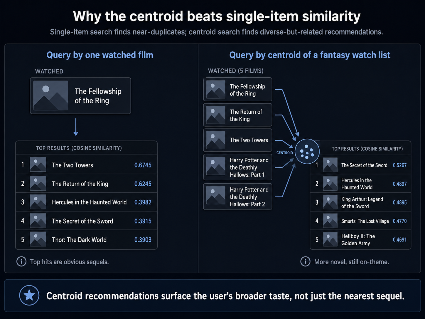
It's worth seeing what you'd have got if you'd just queried by one watched film instead of averaging five. The single-film version of "user B's recommendations" looks like this:
single = np.array(df[df.id == "film-00023"].iloc[0].vector)  # Fellowship of the Ring
single = single / np.linalg.norm(single)
results = vp.vectors.query(
    "movie-recs",
    vector=single.tolist(),
    top_k=5,
    filter={"id": {"$ne": "film-00023"}},
)
for r in results:
    m = r.metadata
    print(f"  {r.score:.4f}  {m.get('title','?')[:40]:<40}  ({m.get('year','?')}, {m.get('genre','?')[:20]})")
results = store.similarity_search_by_vector_with_score(
    single.tolist(),
    k=5,
    filter={"id": {"$ne": "film-00023"}},
)
for doc, score in results:
    m = doc.metadata
    print(f"  {score:.4f}  {m.get('title','?')[:40]:<40}  ({m.get('year','?')}, {m.get('genre','?')[:20]})")
  0.6745  The Lord of the Rings: The Two Towers     (2002, adventure, fantasy)
  0.6245  The Lord of the Rings: The Return of the  (2003, adventure, fantasy)
  0.3982  Hercules in the Haunted World             (1961, adventure)
  0.3915  The Secret of the Sword                   (1985, animation)
  0.3903  Thor: The Dark World                      (2013, superhero)
The top two are the other LOTR films, strong matches by score (0.67, 0.62), but they're sequels to a film the user has already watched. The recommendations only get interesting at position 3, where the score has already dropped to 0.40.
The centroid is a softer query. Scores are flatter (0.47 to 0.53 instead of 0.39 to 0.67), but the first recommendation is already novel rather than being a near-duplicate. That's exactly the trade you want for "here's something else you might enjoy": surface the diverse-but-related, not the obvious.
Now what
You just built a recommendation engine in about 30 lines of Python. The pattern works for anything that's "items embedded in a vector space": products, articles, songs, profile photos, images on a moodboard.
To make it yours:
- Replace the bundled DataFrame with your own (id, vector, plus whatever metadata you'd want to filter on later). Embed your items with whatever model fits the domain.
sentence-transformers/all-MiniLM-L6-v2for text is the default that works almost everywhere. - The watch list is whatever your app has as a "positive signal": purchases, likes, time-on-page, completed views, items added to a playlist. You don't need ratings; presence in the list is the signal.
- Five items in the centroid is a defensible default, not a magic number. Three works. Twenty works. Past about 50, the centroid drifts toward the population mean and recommendations become bland. If your users have very long histories, weight more recent items higher with a weighted average.
- To handle "I liked this and disliked that," subtract the disliked items' centroid from the liked centroid before normalizing. That's the same arithmetic, just signed: it nudges the query away from things the user told you not to recommend.
Read the SDK reference for the full filter operator list and the embeddings 101 concept page for why averaging vectors works as a "taste profile" in the first place.