How auto-optimize picks your index

Choosing an approximate-nearest-neighbor index is, today, a research project per dataset.

There's HNSW. There's IVF, with optional product quantization. There's ScaNN, OPQ, Vamana, PCA-then-cosine, raw scalar quantization, and a half-dozen variations on each. Every one of them has knobs, every one of them has a paper claiming superiority on some benchmark, and every one of them has a different recall and latency profile depending on the shape of the data you point it at.

That's a lot to expect a customer to know.

So we don't.

What we measure

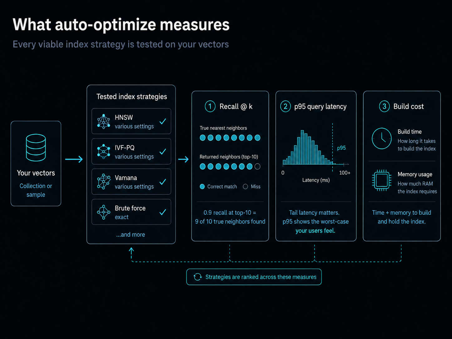
When you create a collection, we sample your vectors and run every viable indexing strategy against that sample. For each strategy and each parameter set, we measure three things:

• Recall @ k. Of the true k nearest neighbors (computed by brute-force as ground truth), what fraction does this strategy return? At top-10, recall of 0.9 means nine of ten "real" neighbors land in the result set.
• p95 query latency. The slow end of typical query response time. Median is misleading on tail-sensitive workloads; p95 is what your users actually feel.
• Build cost. Time and memory required to build the index. Cheap to query but expensive to rebuild changes the math when your data is moving.

These get measured on a sample of your vectors. Not GloVe, not SIFT-1M, not any benchmark dataset. Yours.

The Pareto frontier

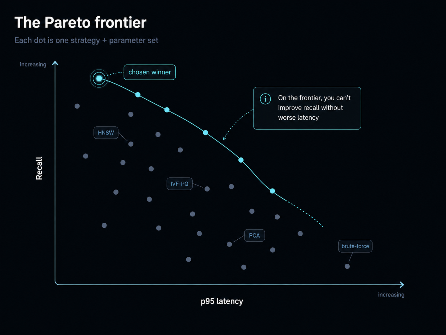
The output is a scatter plot: recall on one axis, p95 latency on the other, one dot per (strategy, parameter set) configuration tested. Some dots are obviously bad: low recall and slow. Some are pleasantly fast but inaccurate. A few sit on the Pareto frontier: the set of configurations where you can't make recall better without making latency worse, and vice versa.

What that looks like in practice on a real run:

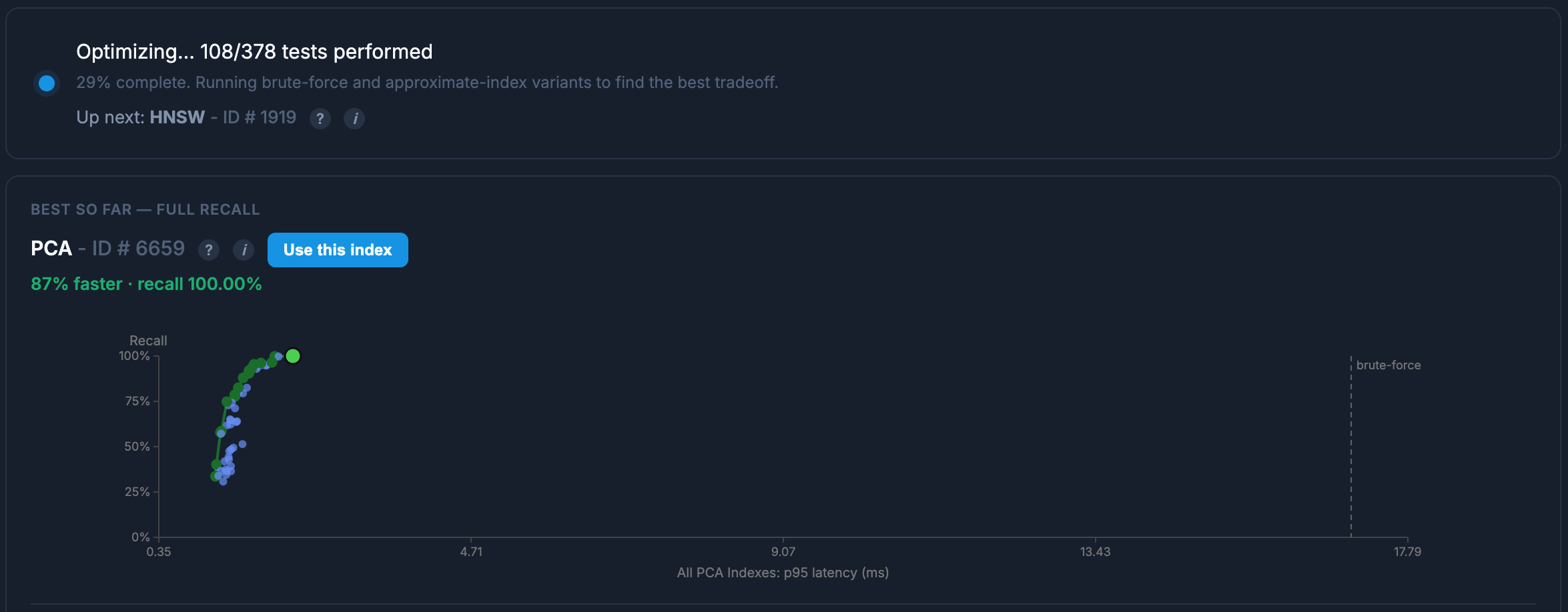
In the run above, 108 of 378 configurations have finished. PCA ID 6659 is the current leader: 100% recall, 87% faster than the brute-force baseline. HNSW ID 1919 is up next. The frontier moves as more results come in. When the run finishes, the chosen winner is whichever point sits highest-and-leftmost on the final frontier.

The strategies we test

Eleven candidates, today:

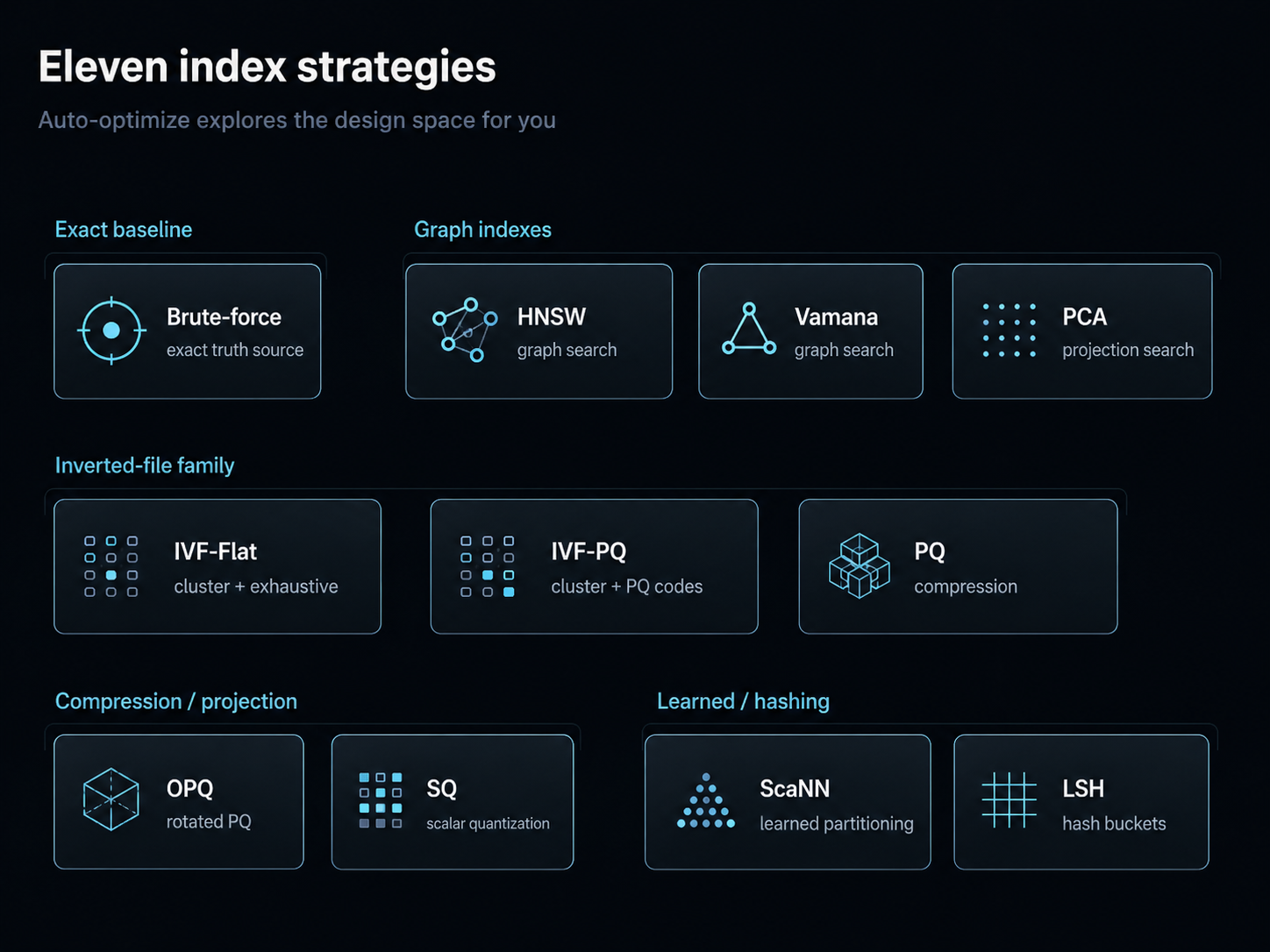
• Brute-force. Scan every vector, return the true top-k. Truth source, and the implicit baseline every other strategy is measured against. Wins when the collection is small enough that the linear cost is below an index's overhead.
• PCA. Project to fewer dimensions and search there. Cheap to build, cheap to query. Wins when the original space has redundant dimensions; loses badly when high-magnitude information lives in the discarded components.
• HNSW. Hierarchical navigable small-world graph. Logarithmic query cost on diverse collections. RAM-hungry: build cost and memory both scale with the connectivity setting.
• Vamana. Single-layer graph with a bounded out-degree, designed for disk-friendly access. The HNSW alternative when memory is tight relative to collection size.
• IVF-Flat. Cluster the data into Voronoi cells, search the n nearest cells exhaustively. Predictable query cost, no compression. Wins when accuracy matters and the data clusters naturally.
• IVF-PQ. IVF clustering plus product-quantized codes inside each cluster. Smaller memory than IVF-Flat at the cost of some recall.
• PQ. Product quantization without the Voronoi step. Splits vectors into chunks, replaces each chunk with the nearest centroid index. Roughly 8x compression with bounded recall loss.
• OPQ. PQ with the space rotated first to minimize quantization error. Better recall than PQ at the same compression. Build cost higher.
• ScaNN. Anisotropic vector quantization with learned hashing, tuned for inner-product search. Wins on dot-product queries where standard tradeoffs are unfavorable.
• SQ (scalar quantization). Compress each dimension independently from float32 to fewer bits. Algorithmically simple, recall hit predictable. The "I just want less memory without rewriting anything" answer.
• LSH (locality-sensitive hashing). Hash similar vectors to the same bucket; query the bucket. Fast in both directions; recall improves with more hash tables. Usually loses to learned methods on real data; we include it because it's a useful baseline and occasionally wins on highly clustered data.

What auto-optimize does with the result

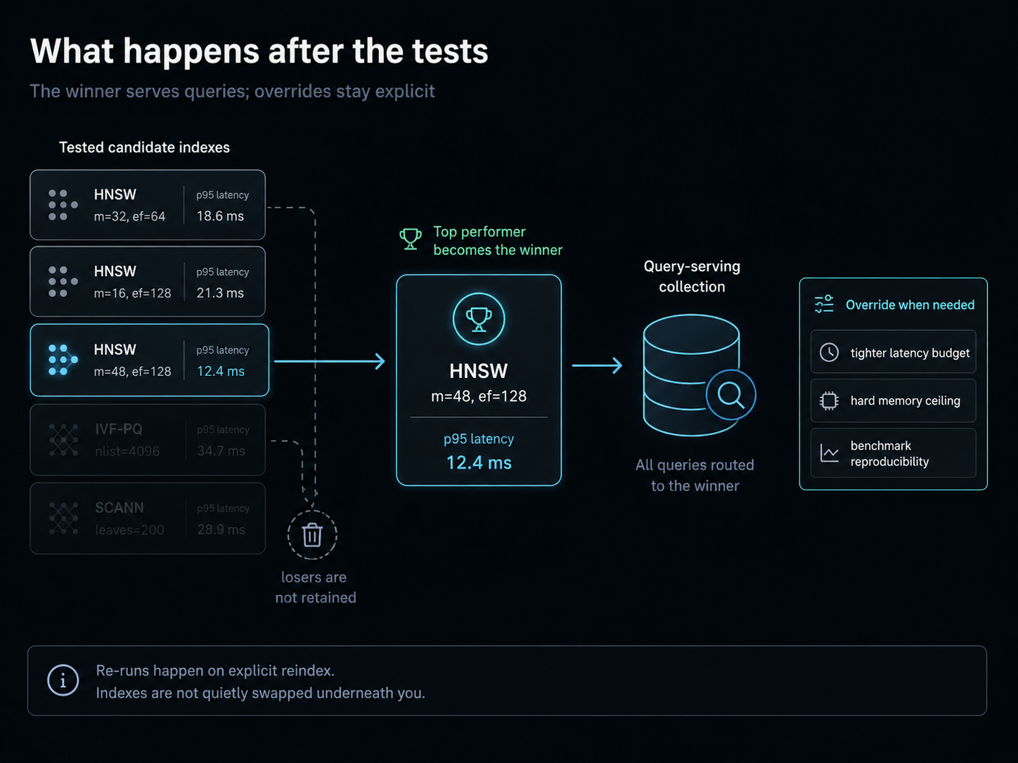
The winner serves your queries. The losers don't get retained: no shadow indexes burning storage, no toggle-it-on-later complexity, no quiet drift between what you thought was running and what's running.

You can browse the frontier in your collection's view: every dot, the live one highlighted, the runner-up gap visible. While optimization is still running, your queries use the best index found so far — we promote a new one whenever we discover a meaningful improvement, so you don't sit on the brute-force baseline for several days waiting for the full sweep. Once optimization completes, the winner is locked: re-runs happen only on explicit reindex, never silent swaps. Index usage is free until the full sweep reaches 100%.

PCA was once a frequent auto-pick. Then a customer pushed in vectors where PCA was throwing away the high-magnitude components and recall fell off a cliff. We don't want that bug to be silent, which is part of the reason we keep brute-force as ground truth and measure recall against it on every run. (See the build-log entry "PCA forgot the magnitudes" for the gory detail.)

When to override

The auto-pick is the right starting point for almost every collection. The real reasons to override are narrow:

• A latency budget tighter than the auto-pick assumes. The frontier picks the highest-recall point under a default latency target. If your real target is lower, pin a faster strategy with worse recall.
• A memory budget you want to enforce. A 16-byte-per-vector PQ variant might be on the frontier but not the winner. If the collection has to fit a specific RAM ceiling, pin it.
• Reproducibility for a benchmark. If you're publishing numbers, you may want the index choice fixed for the experiment.

Overrides are explicit in the SDK and visible in the collection view. Anyone looking at your collection can tell what's running and why.

Further reading

You don't need to read these papers to use Vector Panda. If you'd like to:

• HNSW: Malkov & Yashunin, Efficient and robust approximate nearest neighbor search using Hierarchical Navigable Small World graphs (2018).
• ScaNN: Guo et al., Accelerating Large-Scale Inference with Anisotropic Vector Quantization (Google, 2020).
• Vamana: Subramanya et al., DiskANN: Fast Accurate Billion-point Nearest Neighbor Search on a Single Node (2019).
• FAISS documentation (Meta) covers IVF, PQ, OPQ, and SQ in depth: github.com/facebookresearch/faiss/wiki.

The shape of the field is straightforward once you have the vocabulary. We picked these eleven because they cover the design space well. We're open to adding others if there's a real reason to.